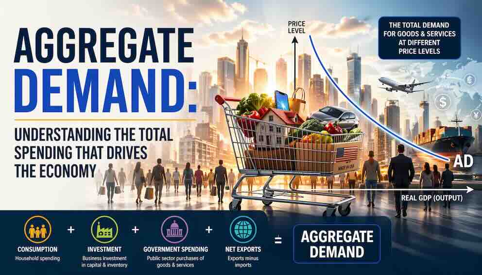
Aggregate Demand: Understanding the Total Spending That Drives the Economy

Introduction: The Force That Moves the Economy

Imagine a giant shopping mall that contains every business in the country—every factory, every farm, every restaurant, every office. Now imagine that every day, all the households, businesses, governments, and foreigners come to this mall to buy what they need. The total amount they spend—on cars, haircuts, computers, bridges, exports—is the economy's aggregate demand. It is the total spending on everything the economy produces. When aggregate demand is strong, businesses are busy, workers are employed, and the economy grows. When aggregate demand is weak, factories sit idle, workers are laid off, and the economy contracts.

Aggregate demand (AD) is one of the most important concepts in macroeconomics. It represents the total quantity of goods and services that all buyers in the economy are willing and able to purchase at different price levels. But here is a crucial distinction: aggregate demand refers to demand for real output, not nominal spending. Even though total dollars spent may rise when prices increase, the quantity of goods and services those dollars can buy may fall. When we talk about the AD curve, we are talking about the real quantity of output demanded at each price level.

Understanding AD is essential for understanding why economies go through booms and recessions, and how fiscal and monetary policy can be used to stabilize the economy. In this tutorial, we will explore the components of aggregate demand, why the AD curve slopes downward, and what causes it to shift. We will use real-world examples from the 2008 financial crisis, the COVID-19 pandemic, and other economic events to bring these concepts to life.

The Components of Aggregate Demand – Who Is Buying?

Aggregate demand is the sum of spending by four groups: households, businesses, governments, and foreigners. This is the same breakdown we encountered in the GDP tutorials, and it is captured by the familiar formula:

AD = C + I + G + (X − M)

Where:

1. C stands for Consumption — spending by households on goods and services.
2. I stands for Investment — spending by businesses on new physical capital (factories, machinery, equipment, housing) and changes in inventories.
3. G stands for Government Spending — spending by federal, state, and local governments on goods and services (but not transfer payments like Social Security).
4. (X − M) stands for Net Exports — exports (X) minus imports (M). This represents spending by foreigners on domestic goods minus domestic spending on foreign goods.

Let us walk through each component slowly, using examples to build intuition.

Consumption: The Spending of Households

Consumption is the largest component of aggregate demand in most economies. In the United States, it typically accounts for about 68 to 70 percent of total spending. Consumption includes everything households spend on: food, rent, gasoline, clothing, healthcare, entertainment, restaurant meals, and so on. When you buy a cup of coffee, that is consumption. When you pay your rent, that is consumption. When you go to the movies, that is consumption. Consumption is the daily engine of the economy.

What determines how much households spend? The most important factor is disposable income—the income people have after taxes. When people have more income, they tend to spend more. But they do not spend all of it; they save some. The proportion of additional income that households spend is called the marginal propensity to consume (MPC) . If the MPC is 0.75, then when income rises by $100, consumption rises by $75. This matters because changes in consumption can have a multiplied effect on aggregate demand—one person's spending becomes another person's income, which leads to further spending. This is the logic of the Keynesian multiplier.

There is also a subtle but important concept called the paradox of thrift. If households collectively try to save more by consuming less, they reduce aggregate demand. This reduction in demand lowers income, which in turn reduces saving. The attempt to save more can actually lead to less saving—a paradox that highlights the importance of understanding AD.

Other factors also matter: household wealth (if stock market or housing prices rise, people feel wealthier and spend more), consumer confidence (if people are optimistic about the future, they spend more), interest rates (if borrowing is cheap, people buy more houses and cars), taxes (lower taxes leave more income to spend), and expectations about future income (if people expect a raise, they may spend more now). It is worth noting that consumption is a flow (a rate of spending per period), while wealth is a stock (an accumulated amount at a point in time). A change in the price level affects the real value of the stock of wealth, which in turn influences the flow of consumption.

Investment: The Spending of Businesses

Investment, in economic terms, does not mean buying stocks or bonds. Those are financial investments—transactions in existing assets—and they do not count toward aggregate demand. Instead, investment in AD refers to spending on new physical capital: factories, machinery, computers, trucks, office buildings, and new housing. It also includes inventory investment—changes in the stock of unsold goods.

Investment is the most volatile component of aggregate demand. When businesses are confident about the future, they invest heavily. When they are uncertain, they pull back. What determines investment? The most important factor is the real interest rate—the nominal interest rate minus expected inflation. When real interest rates are low, borrowing is cheap, and businesses are more likely to finance new projects. When real interest rates are high, investment falls. This is why central banks pay so much attention to inflation expectations: they affect the real interest rate that businesses face.

Business confidence and expectations are also crucial: If firms expect strong future demand, they invest; if they expect a recession, they hold back. Investment also responds to changes in demand—a concept called the accelerator effect. When demand is growing rapidly, firms invest to expand capacity; when demand slows, investment stalls. Technology can drive investment as well; the rise of artificial intelligence, for example, has spurred massive investment in data centers and computing power. Tax policy matters too: investment tax credits and depreciation rules can encourage or discourage spending.

During the 2008 financial crisis, investment collapsed sharply as businesses canceled expansion plans and housing construction ground to a halt. By late 2008, the freeze in credit markets meant that even healthy firms could not borrow to fund new projects. This collapse in investment was both a cause and a consequence of the deep recession that followed, creating a self-reinforcing downward spiral.

Government Spending: The Spending of Governments

Government spending includes purchases of goods and services by federal, state, and local governments. This includes spending on national defense, schools, roads, police, fire services, and public parks. It also includes salaries of government employees—teachers, police officers, firefighters, and administrative staff. What it does not include are transfer payments like Social Security, Medicare, unemployment benefits, or welfare. These are payments to individuals that do not represent a purchase of a new good or service; they simply transfer money from one group to another. When the government sends a Social Security check to a retiree, that money is not counted in G. When the retiree spends that money on groceries, that spending is counted in C.

Government spending is a powerful tool for stabilising the economy. During recessions, when private sector spending (C and I) falls, governments can increase G to offset the decline. A clear example comes from New Zealand's response to the COVID-19 pandemic. In 2020, the government allocated NZ$2.5 billion to an Infrastructure Reference Group with a simple task: find "shovel-ready" projects that could begin within 12 months. The group selected 221 projects spanning transport, environmental restoration, and housing. What makes this example so instructive is that it shows direct government spending on goods and services in action. The government was not sending transfer payments; it was purchasing concrete, steel, engineering services, and construction labour. These purchases created immediate employment, and the wages workers earned supported consumption elsewhere in the economy. The projects also provided long-term benefits: better roads, cleaner rivers, and more housing. This was a pure example of an increase in G – government spending on goods and services – designed to offset the collapse in private demand during the pandemic.

It is also worth noting that government spending interacts with automatic stabilisers. When the economy goes into recession, tax revenues automatically fall and spending on unemployment benefits automatically rises. These automatic changes help cushion the downturn without any new legislation, shifting AD less dramatically than discretionary policy but providing a stabilising force. The New Zealand infrastructure response was a discretionary policy – a deliberate decision to increase spending. It worked alongside automatic stabilisers, such as the rise in unemployment benefits and the fall in tax revenues, to support aggregate demand during the crisis.

Net Exports: Spending from Abroad

Net exports are exports minus imports. Exports (X) are goods and services produced in the country and sold to foreigners. Imports (M) are goods and services produced abroad and purchased by domestic consumers, businesses, or governments. Net exports can be positive (a trade surplus) or negative (a trade deficit). The United States has run a trade deficit for decades, meaning imports exceed exports, so net exports are negative. This subtracts from aggregate demand.

Why do we subtract imports? Because consumption, investment, and government spending all include spending on both domestic and foreign goods. To get aggregate demand for domestically produced goods, we must subtract the value of imports. For example, if a consumer buys a car imported from Japan, that purchase is counted in C, but the car was not produced in the United States. So we subtract the value of the import in the net exports term. This is the trade balance identity: net exports ensure that aggregate demand reflects only spending on domestically produced goods.

What determines net exports? The most important factor is the exchange rate. When the domestic currency is strong (appreciates), exports become more expensive for foreigners and imports become cheaper for domestic consumers. This tends to reduce net exports. When the domestic currency is weak (depreciates), exports become cheaper and imports more expensive, increasing net exports. Foreign income also matters: when our trading partners are growing strongly, they buy more of our exports. Trade policies, such as tariffs and trade agreements, also affect net exports. Expectations about future exchange rates can also influence trade flows, as businesses may delay or accelerate purchases in anticipation of currency movements.

It is also important to note that the exchange rate effect depends on the exchange rate regime. Under a floating exchange rate system (like the United States), the mechanism works as described. Under a fixed exchange rate system, the adjustment may occur through different channels—for example, through changes in domestic prices rather than the exchange rate itself.

Key takeaway: Aggregate demand is the sum of consumption (household spending), investment (business spending on new capital), government spending, and net exports (exports minus imports). Each component is driven by different factors, and together they determine the total demand for domestically produced goods and services.

The Aggregate Demand Curve – What It Shows and How It Is Derived

The aggregate demand curve shows the relationship between the overall price level in the economy and the total quantity of goods and services demanded. It is drawn with the price level on the vertical axis and real GDP (or output) on the horizontal axis. The AD curve slopes downward: when the price level falls, the quantity of goods and services demanded rises; when the price level rises, the quantity demanded falls.

But where does this curve actually come from? It is not simply a "demand curve for everything" in the microeconomic sense. Instead, the AD curve is derived from the underlying relationships between the price level and the components of spending. At each price level, the components of spending—consumption, investment, government spending, and net exports—adjust in response to changes in wealth, interest rates, and exchange rates. The AD curve traces out the total level of output that results from these adjustments. It is, in essence, a general equilibrium outcome of how spending responds to price changes across the economy.

In intermediate macroeconomics, the AD curve is formally derived from the IS-LM model. In that framework, a lower price level increases real money balances (the nominal money supply divided by the price level). This shifts the LM curve to the right, leading to lower interest rates and higher output. The AD curve is the relationship between the price level and the output level that emerges from this process. While we will not go into the full IS-LM derivation here, the intuition is that lower prices increase the real value of money, which stimulates spending through lower interest rates.

Imagine plotting different price levels on the vertical axis. For each price level, we ask: what would be the equilibrium level of output, given how consumption, investment, and net exports respond? The line connecting these points is the AD curve. It slopes downward because of three distinct effects, which we will now explore in detail.

The Wealth Effect

When the overall price level falls, the real value of people's wealth increases. Imagine you have $10,000 in a savings account. If prices fall by 10 percent, your savings can now buy 10 percent more goods and services than before. You feel richer. When people feel richer, they tend to spend more. This increase in consumption causes the quantity of goods and services demanded to rise. Conversely, when the price level rises, the real value of wealth falls, people feel poorer, and they spend less. This is the wealth effect.

It is important to note here the distinction between stocks and flows. Wealth is a stock—an accumulated amount at a point in time. Consumption is a flow—a rate of spending per period. A change in the price level affects the real value of the stock of wealth, which in turn influences the flow of consumption.

The Interest Rate Effect

When the price level falls, households and businesses need less money to conduct their daily transactions. This reduces the demand for money. Assuming the central bank holds the money supply constant (a standard assumption in macroeconomics), a lower demand for money creates an excess supply of money in the money market. To eliminate this excess supply, interest rates fall. People lend out the extra money, and the interest rate adjusts downward.

Lower interest rates make borrowing cheaper, which encourages businesses to invest in new factories and equipment, and encourages households to buy houses and cars. This increase in investment and consumption causes the quantity of goods and services demanded to rise. Conversely, when the price level rises, people need more money for transactions, the demand for money increases, interest rates rise, and investment and consumption fall. This is the interest rate effect.

It is worth noting that what matters for investment is the real interest rate—the nominal interest rate minus expected inflation. If the price level falls and expected inflation also falls, the real interest rate may not fall as much as the nominal rate. This nuance is important for understanding why the interest rate effect can be weaker when inflation expectations are anchored.

The Exchange Rate Effect

When the price level falls in the domestic economy, domestic goods become relatively cheaper compared to foreign goods. This encourages foreigners to buy more of our exports, and it encourages domestic consumers to buy fewer imports (since imports become relatively more expensive). But there is also a second channel: lower domestic prices lead to lower interest rates (as we saw above). Lower interest rates make domestic assets less attractive to foreign investors. Capital flows out of the country, which causes the domestic currency to depreciate. A weaker currency further boosts exports and reduces imports. Both of these channels—the direct price channel and the indirect interest rate/capital flow channel—increase net exports, adding to aggregate demand. Conversely, when the domestic price level rises, interest rates rise, capital flows in, the currency appreciates, and net exports fall. This is the exchange rate effect.

As noted earlier, the strength of this effect depends on the exchange rate regime. Under floating exchange rates (like the United States), the mechanism works through currency movements. Under fixed exchange rates, the adjustment may occur through changes in domestic prices or through changes in foreign exchange reserves.

These three effects work together to make the aggregate demand curve slope downward. A lower price level leads to more spending through wealth effects (consumption), interest rate effects (investment), and exchange rate effects (net exports). A higher price level leads to less spending through the same channels.

Key takeaway: The aggregate demand curve slopes downward because of three effects: the wealth effect (lower prices increase real wealth, boosting consumption), the interest rate effect (lower prices reduce interest rates via the money market, boosting investment), and the exchange rate effect (lower prices and lower interest rates lead to currency depreciation, boosting net exports). The AD curve is derived from the equilibrium output levels that result from these adjustments at different price levels.

Movements Along AD vs Shifts of AD – A Crucial Distinction

One of the most important distinctions in macroeconomics is the difference between a movement along the aggregate demand curve and a shift of the aggregate demand curve.

1. A movement along the AD curve occurs when the price level changes. A fall in the price level increases the quantity of output demanded (a movement down the curve). A rise in the price level decreases the quantity of output demanded (a movement up the curve). The underlying determinants of spending—consumption, investment, government spending, and net exports—remain unchanged; only the price level changes.
2. A shift of the AD curve occurs when something other than the price level changes—when the underlying determinants of C, I, G, or net exports change. A shift to the right means that at every price level, the quantity of goods and services demanded is higher. A shift to the left means that at every price level, the quantity demanded is lower.

Understanding this distinction is essential for analyzing economic events and policy. If the price level falls, we move down the AD curve. But if consumer confidence collapses, the AD curve shifts left—and that shift, not a movement along the curve, is what causes a recession.

Shifts in Aggregate Demand – Moving the Whole Curve

When the price level changes, we move along the AD curve. But when something other than the price level changes—when the underlying determinants of C, I, G, or net exports change—the entire AD curve shifts. Let us examine the factors that cause these shifts.

Factors That Shift Consumption

Several factors can shift consumption independently of the price level. When consumer confidence rises—perhaps because people feel optimistic about their job prospects or the economy—they spend more, shifting AD to the right. When confidence falls, AD shifts left. During the 2008 financial crisis, consumer confidence collapsed, contributing to a sharp leftward shift in AD.

Household wealth also matters. When stock market prices rise or housing values increase, households feel wealthier and spend more, shifting AD right. When asset prices fall, the opposite happens. The dot-com bubble of the late 1990s and the housing bubble of the mid-2000s both boosted consumption through wealth effects until the bubbles burst.

Changes in taxes affect disposable income. When taxes are cut, households have more income to spend, shifting AD right. When taxes are raised, AD shifts left. The effectiveness of tax cuts depends on the marginal propensity to consume—how much of the extra income people actually spend versus save.

Expectations about future income also play a role. If people expect a raise or a bonus, they may increase spending now, shifting AD right. If they expect a recession or job loss, they may save more and spend less, shifting AD left.

Factors That Shift Investment

Investment shifts with interest rates, business confidence, technology, and expected future demand. When the central bank lowers interest rates, borrowing becomes cheaper, and investment tends to increase, shifting AD right. This is the primary channel through which monetary policy works. When the Federal Reserve cut interest rates to near zero during the 2008 crisis and the COVID-19 pandemic, it was trying to shift AD right by boosting investment.

Business confidence is also crucial. Even with low interest rates, businesses will not invest if they are uncertain about future demand. In 2008, investment collapsed despite low rates because businesses feared a prolonged recession. By 2021, with confidence returning, investment surged.

Technological change can drive investment booms. The rise of the internet in the 1990s and artificial intelligence today both spurred massive investment. Expected future demand matters too: when demand is growing rapidly, firms invest to expand capacity—the accelerator effect. When demand slows, investment stalls.

Factors That Shift Government Spending

Government spending shifts with fiscal policy decisions. When Congress and the president increase spending on infrastructure, defense, or education, AD shifts right. When they cut spending, AD shifts left. The American Recovery and Reinvestment Act of 2009, the CARES Act of 2020, and the American Rescue Plan of 2021 were all examples of fiscal stimulus designed to shift AD right. Austerity—cutting government spending—shifts AD left, as seen in the Eurozone debt crisis of the early 2010s.

Automatic stabilizers also play a role. When the economy goes into recession, tax revenues automatically fall and spending on unemployment benefits automatically rises. These changes help cushion the downturn without new legislation, shifting AD right automatically during recessions and left during booms.

Factors That Shift Net Exports

Net exports shift with exchange rates, foreign income, and trade policies. When the domestic currency depreciates (weakens), exports become cheaper and imports more expensive, increasing net exports and shifting AD right. When the dollar strengthened in the mid-2010s, net exports fell, shifting AD left.

When foreign economies are growing strongly, they buy more of our exports, shifting AD right. When they are in recession, our exports fall, shifting AD left. The 2008 financial crisis was global; as economies around the world contracted, U.S. exports fell sharply.

Trade policies such as tariffs, quotas, and trade agreements also affect net exports. The Trump administration's tariffs on Chinese goods in 2018 and 2019 reduced trade between the two countries, affecting net exports.

The Role of Expectations Across All Components

Modern macroeconomics emphasizes that expectations are a driver of all components of AD. Expected future income affects consumption. Expected future profits affect investment. Expected future exchange rates affect net exports. Expected future policy affects government spending decisions (through anticipation). And expected inflation affects whether people spend now or later. When expectations shift, the AD curve shifts—sometimes dramatically. This is why central banks spend so much effort on "forward guidance": managing expectations about future policy to influence AD today.

Putting It All Together – AD and the Economy

Aggregate demand is not just a theoretical concept; it is the lens through which economists and policymakers view the economy. When the economy is in a recession, it is often because AD is too low. Factories are running below capacity, workers are unemployed, and businesses are not investing. In this situation, policymakers try to increase AD—through lower interest rates (monetary policy) or increased government spending and tax cuts (fiscal policy).

When the economy is overheating—when demand is too strong relative to the economy's capacity to produce—inflation rises. In this situation, policymakers try to reduce AD—through higher interest rates or reduced government spending and tax increases.

In the short run, shifts in AD affect both output and prices. An increase in AD raises output and employment but also puts upward pressure on prices. A decrease in AD lowers output and employment but also reduces inflationary pressure. In the long run, however, the economy's productive capacity (aggregate supply) determines output, and shifts in AD primarily affect prices. This distinction—between short-run and long-run effects—is a central theme in macroeconomics.

The 2008 financial crisis was a classic case of insufficient AD. The collapse in housing wealth, business confidence, and global trade caused a massive leftward shift in AD. The response—zero interest rates and fiscal stimulus—was aimed at shifting AD back to the right.

The COVID-19 pandemic was similar: a sudden collapse in consumption and investment caused AD to plummet. Again, policymakers responded with massive stimulus.

The 2021–2023 inflation surge was a case of excessive AD. With households flush with cash from stimulus, low interest rates, and pent-up demand, AD shifted sharply to the right. Supply could not keep up, and prices rose. The Federal Reserve's response—raising interest rates—was aimed at cooling AD.

Understanding aggregate demand helps us understand these events. It provides a framework for thinking about why economies boom and bust, and how policy can stabilize them. It is not the whole story—supply also matters, as we will see in the next tutorial—but it is an essential foundation.

Key takeaway: Aggregate demand is a central concept in macroeconomics. When AD is too low, the economy experiences recession and unemployment. When AD is too high, it experiences inflation. Policymakers use monetary and fiscal policy to shift AD to achieve stable growth and low inflation. In the short run, AD shifts affect output; in the long run, they primarily affect prices.

Conclusion: The Total Spending That Shapes Our Lives

We began this tutorial with the image of a giant shopping mall where all the spending in the economy takes place. That image captures the essence of aggregate demand: it is the total spending on everything the economy produces. When that spending is strong, businesses thrive, workers are employed, and the economy grows. When it is weak, factories close, people lose jobs, and the economy contracts.

We have explored the four components of aggregate demand: consumption, investment, government spending, and net exports. We have seen how each component is driven by different factors—income, wealth, confidence, interest rates, exchange rates, policy decisions, and expectations—and how together they determine the total demand for domestically produced goods and services.

We have learned that the aggregate demand curve is derived from the equilibrium output levels that result from spending adjustments at different price levels. We have understood why it slopes downward, examining the wealth effect (lower prices make people feel richer), the interest rate effect (lower prices reduce interest rates via the money market, boosting investment), and the exchange rate effect (lower prices and lower interest rates lead to currency depreciation, boosting net exports). We have drawn the crucial distinction between movements along the AD curve (caused by price level changes) and shifts of the AD curve (caused by changes in C, I, G, or net exports). And we have examined the factors that cause AD to shift—changes in consumer confidence, wealth, taxes, interest rates, business confidence, technology, government spending, exchange rates, foreign income, and expectations—using real-world examples from the 2008 financial crisis, the COVID-19 pandemic, and the 2021–2023 inflation surge.

Aggregate demand is not just a measure of spending. It is the transmission mechanism through which expectations, policy, and global conditions shape the entire economy. When a government announces a stimulus package, it is trying to shift AD. When a central bank signals future interest rate changes, it is trying to manage expectations to influence AD today. When businesses decide whether to build a new factory, they are responding to their expectations of future AD. Understanding aggregate demand means understanding the forces that create jobs, determine incomes, and shape the economic world we all inhabit. It is the expression of confidence, the reflection of collective behavior, and the force that moves the economy—sometimes gently, sometimes with great force.