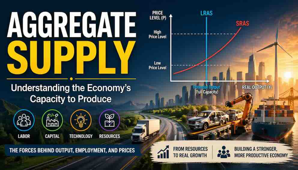
Aggregate Supply: Understanding the Economy's Capacity to Produce

Introduction: The Other Side of the Economy

Imagine a factory that produces cars. It has a certain number of workers, a certain number of machines, and a certain level of technology. At any given moment, the factory can produce only so many cars. It can run overtime, hire temporary workers, or push machines a little harder, but there is a limit. If orders pour in—if aggregate demand surges—the factory cannot instantly double its output. It needs time to hire more workers, build new factories, and install new equipment. And if costs rise—if the price of steel jumps or wages increase—the factory may produce less, or it may raise its prices to cover the higher costs.

This is the story of aggregate supply (AS). While aggregate demand represents the total spending in the economy, aggregate supply represents the total output that firms are willing and able to produce at different price levels. Economists represent aggregate supply using a graph with the overall price level on the vertical axis and real output (GDP) on the horizontal axis. This is different from standard supply curves in microeconomics. Instead of the price of a single good, we are dealing with the average price of all goods in the economy.

Understanding AS is essential for understanding why economies cannot simply grow as fast as demand might want them to, why there are limits to how much the economy can produce without causing inflation, and why supply shocks—like oil price spikes or pandemics—can have such profound effects.

In this tutorial, we will explore the two distinct concepts of aggregate supply: short-run aggregate supply (SRAS) , where some prices and wages are sticky and do not adjust instantly, and long-run aggregate supply (LRAS) , where all prices and wages have fully adjusted and the economy operates at its full capacity. We will examine why wages and prices are rigid—the reasons they do not adjust instantly to changes in demand—and explore the factors that cause the aggregate supply curves to shift. Using real-world examples from the 1970s oil shocks, the 2008 financial crisis, the COVID-19 pandemic, and the 2021–2023 inflation surge, we will see how AS shapes the economy's response to shocks and policy.

The Two Time Horizons – Short-Run vs Long-Run Aggregate Supply

When economists talk about aggregate supply, they distinguish between the short run and the long run. This distinction is not about a fixed number of months or years; it is about whether prices and wages have had time to fully adjust to changes in the economy.

Short-Run Aggregate Supply: A World of Sticky Prices and Wages

In the short run, many prices and wages are sticky – they do not adjust immediately to changes in demand. A restaurant cannot change its menu prices every time a customer walks in. A worker's salary is set by contract, often for a year or more. A factory's supply contracts lock in prices for raw materials months in advance.

Because of this stickiness, when the overall price level rises, firms find that their costs (wages, raw materials) do not rise immediately. Their profits increase, so they are willing to produce more. This gives the short-run aggregate supply curve its distinctive upward slope: as the price level rises, the quantity of goods and services supplied increases.

A deeper way to think about short-run aggregate supply is that output rises when actual inflation turns out higher than expected inflation. When prices rise more than workers and firms anticipated, real wages fall temporarily, and firms expand production. Workers, who expected a certain price level, see their real wages decline without having negotiated for higher pay. Firms take advantage of the lower real labour cost to increase output. Conversely, when actual inflation is lower than expected, real wages rise, and firms reduce production. This expectations-augmented view is central to modern macroeconomics and explains why the SRAS curve is upward-sloping.

Why does the SRAS curve slope upward? There are three main explanations, all rooted in the idea that some prices adjust more slowly than others.

The Sticky-Wage Theory

Wages are often set by contracts that last for a year or more. Unions negotiate multi-year agreements. Many workers receive annual salary reviews. Even for workers without formal contracts, there are social norms against cutting wages. Workers resist pay cuts, and employers are reluctant to impose them for fear of damaging morale or losing good employees. This phenomenon is sometimes called "downward wage rigidity" – wages can go up easily, but they rarely go down.

Because wages are sticky, they do not adjust instantly when the overall price level changes. Suppose the overall price level rises unexpectedly. The wages firms pay are fixed by contracts, so the real wage – the wage adjusted for inflation – falls. Labour becomes cheaper for firms, so they hire more workers and increase production. Conversely, if the price level falls unexpectedly, real wages rise, labour becomes more expensive, and firms reduce production. Because wages are sticky, changes in the price level affect firms' costs and their willingness to produce.

The COVID-19 pandemic provided a striking demonstration of downward wage rigidity. In 2020, as lockdowns brought large parts of the economy to a halt, unemployment soared. Yet wages did not fall. In fact, average wages actually rose sharply in the early months of the pandemic. This increase was not because employers were handing out raises. Rather, it was caused by a change in the composition of the workforce: as employers laid off lower-paid workers in sectors like hospitality and retail, the average wage of those still employed rose because higher-paid workers made up a larger share of the workforce.

More importantly, when the economy began to recover and employers scrambled to rehire, wages did not fall back to pre-pandemic levels. Instead, nominal wages continued to rise. Pay for workers who changed jobs in the leisure and hospitality sector surged by over 15 per cent. Firms did not cut wages to reduce costs during the downturn. Instead, they laid off workers. And when demand returned, they raised wages sharply to attract new hires. The adjustment to the shock happened through quantities (employment) rather than through prices (wages). This is downward wage rigidity in action: wages can go up easily, but they rarely go down, even during a severe economic crisis.

The Sticky-Price Theory

Not all firms adjust their prices instantly. Some have "menu costs" – the costs of changing prices, such as printing new menus, updating websites, or renegotiating contracts. When the overall price level rises, firms with sticky prices find their goods relatively cheaper, so they sell more. To meet the higher demand, they increase production. This contributes to the upward slope of SRAS.

Beyond menu costs, a deeper form of price stickiness comes from what economists call administered prices. This term, introduced by economist Gardiner Means in the 1930s, refers to prices that are set by administrative decision rather than by the moment-to-moment forces of supply and demand. Means observed that during the Great Depression, many industrial prices did not fall as classical economic theory predicted. Instead, they remained stable, and the adjustment to falling demand happened through falling sales, production, and employment.

Subsequent research has confirmed that administered pricing is not a relic of the 1930s but a normal feature of modern economies. Surveys conducted across many countries have found that 70 to 85 per cent of industrial prices in the United States are set using cost-based "markup" pricing rather than responding to demand fluctuations. Similar patterns have been documented in the Eurozone (54 per cent), Portugal (65 per cent), Germany (73 per cent), France (52 per cent), Italy (52 per cent), Japan (45 per cent), and Australia (59 per cent). Firms set prices based on their costs plus a fixed profit margin. They change prices only when their costs change, not when demand rises or falls. This means that for a large portion of the economy, prices are sticky by design, not because of menu costs alone.

During the COVID-19 pandemic, this administered pricing behaviour was visible. Many businesses faced a sudden drop in demand. Some responded by cutting prices, but many did not. Restaurants kept their menu prices stable even as fewer customers came. This stickiness meant that the adjustment to the shock happened through quantities (fewer meals sold) rather than through prices. The administered prices literature helps explain why: for many firms, prices are set as a markup on costs, not as a response to demand. When demand falls, they do not cut prices; they simply sell less.

The Misperceptions Theory

Sometimes, firms do not know whether a change in the price of their product reflects a change in overall demand or a change in demand for their specific product. If the overall price level rises, a firm might mistakenly believe that the demand for its product has increased and respond by producing more. It takes time for firms to realise that the price increase is general, not specific to them. This misperception contributes to short-run supply responsiveness.

These three theories all imply that in the short run, when the price level rises, output rises; when the price level falls, output falls. The SRAS curve slopes upward.

Long-Run Aggregate Supply: The Full Capacity of the Economy

In the long run, all prices and wages have had time to adjust. Contracts expire and are renegotiated. Menu costs are paid. Firms correct their misperceptions. In the long run, the economy produces at its full capacity – the level of output consistent with full employment of labour and capital, given the available technology. Economists refer to this level as potential output, also called full-employment output or the natural level of output.

The long-run aggregate supply curve is vertical. Why? Because in the long run, the economy's output is determined by its productive capacity – the quantity of labour, the stock of capital, and the level of technology – not by the price level. Changes in the price level do not affect these real factors. If the price level doubles, wages and other costs will eventually double as well, leaving firms with no incentive to change production. The economy will produce the same amount of output regardless of the price level.

This idea – that changes in the price level do not affect real output in the long run – is known as the long-run neutrality of money. It is one of the core principles of macroeconomics. It tells us that while monetary policy can influence output in the short run by affecting demand, it cannot permanently increase the economy's productive capacity. Only improvements in labour, capital, and technology can do that.

If the economy is producing above or below potential output, adjustments in wages and prices will gradually bring it back. This is the self-correcting mechanism of the economy. If output is above potential, wages will eventually rise, shifting SRAS left and bringing output back down. If output is below potential, wages will eventually fall, shifting SRAS right and bringing output back up. This self-correction is why the long run is different from the short run.

Think of it this way: the long-run aggregate supply curve represents the economy's "speed limit." Just as a car cannot exceed its top speed no matter how hard you press the accelerator (without risking damage), the economy cannot sustainably produce beyond its potential without causing inflation. In the long run, output is determined by supply-side factors, not by demand.

Key takeaway: Short-run aggregate supply (SRAS) slopes upward because wages and prices are sticky. A deeper view is that output rises when actual inflation exceeds expected inflation. Long-run aggregate supply (LRAS) is vertical because in the long run, output is determined by the economy's productive capacity – labour, capital, and technology – not by the price level. This is known as the long-run neutrality of money, and the economy self-corrects toward potential output over time.

Shifts in Short-Run Aggregate Supply – When the Supply Curve Moves

The short-run aggregate supply curve can shift. A shift to the right means that at every price level, firms are willing to produce more. A shift to the left means that at every price level, they are willing to produce less. It is crucial to distinguish this from a movement along the curve: a change in the price level causes a movement along the SRAS curve, while changes in costs or expectations cause the entire curve to shift.

What causes these shifts? They can be grouped into two main categories: cost shocks and expectations and structural factors.

Cost Shocks: Changes in Input Prices

The most important factor affecting SRAS is the price of inputs—especially labor, energy, and raw materials. When input prices rise, firms' costs increase. They respond by reducing production at every price level, shifting SRAS to the left. When input prices fall, SRAS shifts to the right.

The 1970s Oil Shocks. In 1973 and again in 1979, the Organization of Petroleum Exporting Countries (OPEC) imposed an oil embargo, causing the price of crude oil to quadruple. Oil is a key input for almost every industry—transportation, manufacturing, heating, and electricity generation. The sharp increase in energy costs caused the SRAS curve to shift sharply to the left. The result was stagflation—a combination of high inflation (because costs rose) and high unemployment (because output fell). This was a classic negative supply shock.

The 2008 Oil Price Spike. Before the financial crisis, oil prices rose to nearly $150 per barrel. This increase in input costs shifted SRAS left, contributing to inflationary pressures even before the crisis hit.

The 2021–2023 Supply Chain Disruptions. During the pandemic, supply chains were severely disrupted. Shortages of semiconductors, shipping containers, and labor caused input costs to rise for many industries. This shifted SRAS left, contributing to the inflation surge.

Expectations and Structural Factors

Changes in Expected Inflation. If firms expect higher inflation in the future, they may raise prices now in anticipation. This shifts SRAS left. If they expect lower inflation, they may be more cautious about raising prices, shifting SRAS right. Expectations matter because they influence wage negotiations and price-setting behavior. This is why central banks work so hard to "anchor" inflation expectations—to keep them stable so that they do not become a source of supply shocks.

Changes in Labor Supply and Productivity. The availability of labor affects SRAS. If immigration increases, or if more people enter the workforce, the labor supply expands, and SRAS shifts right. If the labor force shrinks, SRAS shifts left. Similarly, productivity—the output per worker—affects SRAS. When productivity rises, firms can produce more with the same inputs, shifting SRAS right. When productivity falls, SRAS shifts left.

Temporary vs Permanent Supply Shocks

It is important to distinguish between temporary supply shocks and permanent changes. A temporary shock—like a harsh winter that disrupts transportation—shifts SRAS left in the short run, but the curve returns to its original position once the shock passes. A permanent change—like a new technology or a change in immigration policy—shifts LRAS as well as SRAS. Understanding the persistence of a shock is crucial for policy. If a supply shock is temporary, policymakers may be able to "look through" it. If it is permanent, they must adjust.

Key takeaway: Short-run aggregate supply shifts left when input prices rise, expected inflation rises, or labor supply or productivity falls. It shifts right when input prices fall, expected inflation falls, or labor supply or productivity rises. The 1970s oil shocks and the 2021–2023 supply chain disruptions are classic examples of negative supply shocks that shifted SRAS left, creating stagflation.

Shifts in Long-Run Aggregate Supply – Growing the Economy's Capacity

Long-run aggregate supply represents the economy's potential output—the maximum sustainable level of production given available resources and technology. Because LRAS is vertical, shifts in LRAS represent changes in the economy's capacity to produce. These shifts are driven by changes in the factors that determine potential output.

Changes in Labor Supply

The quantity of labor available affects potential output. When the population grows, or when more people enter the workforce (for example, as women entered the labor force in the second half of the twentieth century), LRAS shifts right. When the labor force shrinks—as it will in many advanced economies as populations age—LRAS shifts left.

Changes in Physical and Human Capital

Investment in new factories, machinery, and infrastructure increases the stock of physical capital, shifting LRAS right. Investment in education and training increases human capital—the skills and knowledge of workers—also shifting LRAS right. This is why economists emphasize investment as a driver of long-run growth.

The Post-World War II Boom. After World War II, the United States experienced a period of rapid investment in manufacturing, infrastructure, and education. The GI Bill sent millions of veterans to college, boosting human capital. The interstate highway system was built, boosting physical capital. These factors shifted LRAS right, contributing to decades of strong growth.

The Rise of China. Over the past forty years, China has experienced massive shifts in LRAS as it industrialized, invested in education and infrastructure, and integrated into the global economy. The result has been a sustained rightward shift in China's LRAS, lifting hundreds of millions of people out of poverty.

Changes in Technology

Technological progress is the most important driver of long-run growth. New technologies allow workers to produce more with the same inputs. The invention of the steam engine, the electric motor, the computer, and the internet all shifted LRAS right. Today, advances in artificial intelligence, biotechnology, and renewable energy are shifting LRAS right. AI, in particular, has the potential to be a massive positive LRAS shock, boosting productivity across many industries.

The Productivity Slowdown. In the 1970s, productivity growth slowed in many advanced economies. The reasons are debated—some point to the oil shocks, others to a slowdown in technological innovation—but the effect was a slowdown in the rightward shift of LRAS. This contributed to the stagflation of the era.

Changes in Natural Resources

The availability of natural resources affects potential output. The discovery of new oil fields, for example, shifts LRAS right. Depletion of resources shifts LRAS left. Climate change—through its effects on agriculture, infrastructure, and labor productivity—could shift LRAS left in the long run if not addressed.

Institutions and Policy

The quality of institutions—property rights, rule of law, regulatory efficiency—affects LRAS. Countries with strong institutions tend to have higher potential output. Policies that encourage innovation, investment, and education shift LRAS right. Policies that discourage them shift LRAS left.

Key takeaway: Long-run aggregate supply shifts right when labor supply, capital stock, technology, or resource availability increases. It shifts left when these factors decrease. Investment in human and physical capital, technological progress, and strong institutions are the engines of long-run growth.

Putting It All Together – AS and the Economy

Aggregate supply and aggregate demand together determine the economy's output and price level. In the short run, the intersection of AD and SRAS determines output and prices. Because SRAS slopes upward, changes in AD affect both output and prices. An increase in AD raises output and prices; a decrease in AD lowers output and prices.

In the long run, however, the economy adjusts. If AD increases, output initially rises above potential, and unemployment falls below the natural rate. But eventually, wages and prices adjust. Workers demand higher wages, raising firms' costs. The SRAS curve shifts left until output returns to potential and prices have risen. The long-run effect of an increase in AD is higher prices, not higher output.

This creates a fundamental challenge for policymakers. Policies that boost demand—like lower interest rates or increased government spending—can stabilize the economy in the short run, reducing unemployment and boosting output during recessions. But without improvements in aggregate supply, sustained demand stimulus risks generating inflation rather than sustainable growth. In the long run, output is determined by supply-side factors. To increase the economy's capacity—to shift LRAS right—policymakers must invest in education, infrastructure, technology, and institutions.

Hysteresis: When Recessions Leave Scars

One important nuance is the concept of hysteresis—the idea that deep recessions can cause permanent damage to the economy's productive capacity. When workers lose jobs for extended periods, their skills may atrophy. When young people graduate into a recession, their lifetime earnings may be permanently lower. When firms close during a downturn, the capital they used may be lost forever. In these cases, a temporary demand shock can shift LRAS left, turning a cyclical problem into a structural one. This is why some economists argue that policymakers should be aggressive in fighting recessions: to prevent temporary downturns from becoming permanent scars.

Real-World Example: The COVID-19 Pandemic. The pandemic was a massive negative supply shock. It disrupted labor supply (workers stayed home), capital utilization (factories closed), and supply chains (global trade ground to a halt). SRAS shifted left. At the same time, fiscal stimulus shifted AD right. The result was a sharp increase in the price level—inflation—and a recovery in output that was constrained by supply-side bottlenecks. This episode illustrates the interaction of AD and AS in real time.

Real-World Example: The 2008 Financial Crisis. The financial crisis was primarily a demand shock—a collapse in consumption and investment shifted AD left. But it also had supply-side effects through hysteresis. As firms closed and workers lost skills, potential output fell. LRAS shifted left, contributing to the slow recovery. This is why the recovery from the 2008 crisis was so sluggish compared to previous recessions.

Key takeaway: In the short run, AD and SRAS determine output and prices. In the long run, output returns to potential, determined by LRAS. Policymakers can influence output in the short run through demand-side policies, but long-run growth depends on supply-side factors. Hysteresis reminds us that deep recessions can cause permanent damage to the economy's productive capacity.

Conclusion: The Limits and Potential of the Economy

We began this tutorial with the image of a factory that cannot produce more than its capacity allows. That image captures the essence of aggregate supply: the economy has limits. It cannot grow faster than its workforce, its capital stock, and its technology allow without causing inflation. But those limits are not fixed. Through investment, education, and innovation, we can expand them. We can shift the long-run aggregate supply curve to the right, creating the capacity for higher living standards.

This creates a fundamental tension for policymakers. In the short run, they can use demand-side tools—monetary and fiscal policy—to stabilize the economy, cushioning the impact of recessions and keeping output near potential. But in the long run, sustained growth depends on supply-side factors: the skills of the workforce, the quality of capital, the pace of innovation, and the strength of institutions. The best policy combines both: using demand-side tools to stabilize the economy in the short run while investing in the supply-side foundations of long-run growth.

Aggregate supply is the other side of the economy—the side that reminds us that there are limits to what the economy can produce. But it is also the side that reminds us that those limits can be expanded. When we invest in education, we are shifting LRAS right. When we build infrastructure, we are shifting LRAS right. When we develop new technologies, we are shifting LRAS right. Understanding aggregate supply helps us understand not only why economies experience recessions and inflation but also how they grow over the long term. The limits are real, but they are not permanent. They are the starting point, not the destination.