The Phillips Curve: Why Governments Once Thought They Could Trade Inflation for Unemployment – And Why They Were Wrong

The Discovery That Changed Macroeconomics

In 1958, a New Zealand-born economist named A.W. Phillips published a paper that would reshape how governments thought about the economy for two decades. Phillips had done something simple but powerful: he plotted data on wage inflation – the rate at which wages were rising – and unemployment in the United Kingdom over nearly a century, from 1861 to 1957. When he looked at the scatter plot of points, a clear pattern emerged. In years when unemployment was low, wages tended to rise quickly. In years when unemployment was high, wages tended to rise slowly or even fall. The relationship was not perfect – there were points scattered around – but the downward slope was unmistakable. Phillips had discovered a trade-off: you could have low unemployment, but you would pay for it with higher wage inflation. Or you could have low wage inflation, but you would pay for it with higher unemployment. You could not have both.

This discovery was electrifying for policymakers. For decades, governments had felt powerless in the face of the business cycle. Recessions brought high unemployment and human suffering. Booms brought inflation that eroded savings. There seemed to be no way to escape this cycle. But the Phillips Curve suggested something extraordinary: maybe governments could choose their preferred point on the trade-off. If a government wanted lower unemployment, it could accept higher inflation. If it wanted lower inflation, it could accept higher unemployment. The Phillips Curve appeared to be a menu of policy choices, and for a generation of politicians and economists, that menu was irresistible.

The logic behind the original Phillips Curve is intuitive. When unemployment is low, the labour market is tight. Businesses that want to hire more workers cannot find them easily because most people who want jobs already have them. To attract workers from other firms, businesses must offer higher wages. Those higher wages are a cost of production, and businesses pass those higher costs along to their customers by raising prices. So low unemployment leads to rising wages, which leads to rising prices – inflation. Conversely, when unemployment is high, there are many workers competing for few jobs. Workers have little bargaining power, so wages rise slowly or not at all. With stable labour costs, prices also remain stable. The trade-off seemed to be a fact of economic life.

A Note on Wage Inflation vs Price Inflation: Phillips originally studied wage inflation (how fast wages are rising). But policymakers care about price inflation (how fast the cost of living is rising). The two are closely linked because wages are a major cost for most businesses. When wages rise quickly, businesses raise prices to protect their profits. So the relationship that Phillips found between unemployment and wage inflation also holds – with some modification – between unemployment and price inflation. Modern economics focuses on price inflation because that is what matters for household budgets and central bank targets.

Key Takeaway – The Original Discovery: A.W. Phillips found a negative relationship between unemployment and wage inflation in UK data from 1861 to 1957. Low unemployment was associated with high wage inflation; high unemployment was associated with low wage inflation. This suggested a policy trade-off that governments found irresistible.

The Short-Run Phillips Curve – A Temporary Gift for Policymakers

The original Phillips Curve described a relationship that held over long periods of history. But economists soon realised that the trade-off was not stable. It could shift. This led to the distinction between the short-run Phillips Curve (SRPC) and the long-run Phillips Curve (LRPC) , a distinction that is absolutely central to modern macroeconomics.

The short-run Phillips Curve is downward sloping. It shows that in the short run, when inflation expectations are fixed, there is a trade-off between inflation and unemployment. If the government uses expansionary policy – cutting taxes, increasing spending, or having the central bank lower interest rates – it can boost aggregate demand. Higher demand means businesses need to produce more, so they hire more workers. Unemployment falls. But as unemployment falls, the labour market tightens, and wages start to rise. Businesses raise prices to cover higher labour costs. Inflation rises. In the short run, the government has successfully traded higher inflation for lower unemployment.

Why does this only work in the short run? The answer lies in adaptive expectations. Adaptive expectations means that people form their expectations about future inflation based on what inflation has been in the recent past. If inflation has been low for a long time, people expect it to stay low. When the government launches an expansionary policy and inflation begins to rise, people do not immediately adjust their expectations. Workers do not immediately demand huge wage increases because they still expect inflation to be low. Businesses do not immediately raise prices by the full amount because they still expect their costs to be stable. This delay – this stickiness of expectations – is what creates the short-run trade-off. The government gets a temporary window where it can reduce unemployment before expectations catch up.

The real-world example of this thinking was the United States in the 1960s. President Lyndon B. Johnson's administration pursued expansionary fiscal policy – tax cuts and increased spending on the Great Society programmes and the Vietnam War – while the Federal Reserve kept interest rates low. Unemployment fell from around five per cent in the early 1960s to under four per cent by the late 1960s. Inflation began to rise, from about one per cent to nearly five per cent. For a while, it seemed like the Phillips Curve trade-off was working exactly as advertised. The government had bought lower unemployment at the cost of somewhat higher inflation, and many people thought that was a reasonable bargain.

Key Takeaway – Short-Run Phillips Curve: The SRPC slopes downward. When inflation expectations are fixed, expansionary policy can temporarily reduce unemployment at the cost of higher inflation. This works because people do not immediately adjust their expectations (adaptive expectations).

The Expectations-Augmented Phillips Curve – The Formal Model

To understand modern thinking about the Phillips Curve, we need a simple equation that captures everything we have discussed. This is called the expectations-augmented Phillips Curve, and it is one of the most important equations in macroeconomics. Here it is:

π = π^e − β (u − u^*) + s

Let us break this down piece by piece. The symbol π (the Greek letter pi) stands for the actual inflation rate. The symbol π^e stands for expected inflation – what people think inflation will be. The symbol u stands for the actual unemployment rate. The symbol u^* (u-star) stands for the natural rate of unemployment, also called the NAIRU (Non-Accelerating Inflation Rate of Unemployment). The Greek letter β (beta) is a positive number that tells us how sensitive inflation is to changes in unemployment. The symbol s stands for supply shocks – things like oil price spikes or pandemic disruptions that directly affect inflation.

Now let us see what this equation tells us. The term −β (u − u^) means that when unemployment is below the natural rate (u is less than u^), this term becomes positive (because a negative times a negative is positive), which pushes inflation up. When unemployment is above the natural rate (u is greater than u^*), this term becomes negative, which pushes inflation down. The expected inflation term π^e means that if people expect higher inflation, actual inflation will be higher at any given level of unemployment. The supply shock term s means that an oil price spike or a pandemic disruption adds directly to inflation regardless of unemployment.

This equation unifies everything in the Phillips Curve story. When expected inflation π^e is fixed, the equation shows a downward-sloping relationship between inflation and unemployment – the short-run Phillips Curve. But when expected inflation changes, the entire curve shifts. If people expect higher inflation, the curve shifts up. If they expect lower inflation, it shifts down. In the long run, expectations adjust fully. If inflation has been running at five per cent for years, people will come to expect five per cent. In the long run, π = π^e. Plugging that into the equation, we get π = π − β (u − u^*) + s. Cancel π from both sides, and we get 0 = −β (u − u^*) + s, or β (u − u^*) = s. Without supply shocks (s = 0), this gives u = u^*. The long-run Phillips Curve is vertical at the natural rate of unemployment. Supply shocks can shift the long-run relationship, but in the absence of persistent supply shocks, there is no long-run trade-off.

The Accelerationist Insight: The equation also reveals a crucial fact that is often missed. To keep unemployment below the natural rate (u < u^), the term −β (u − u^) is positive. To keep actual inflation π constant, expected inflation π^e must keep rising to match the actual inflation. In other words, to keep unemployment below the natural rate, inflation must keep accelerating year after year. Constant inflation means unemployment at the natural rate. Falling inflation means unemployment above the natural rate. Rising inflation means unemployment below the natural rate. This is why the natural rate is called the NAIRU – the Non-Accelerating Inflation Rate of Unemployment.

Key Takeaway – The Equation: π = π^e − β (u − u^*) + s. This shows that actual inflation depends on expected inflation, the gap between actual unemployment and the natural rate, and supply shocks. In the long run, expectations adjust, and unemployment returns to the natural rate – no long-run trade-off.

The Long-Run Phillips Curve – The Vertical Reality

The insight that there is no long-run trade-off between inflation and unemployment was developed independently by Milton Friedman and Edmund Phelps in the late 1960s, and it fundamentally changed macroeconomics. They argued that there is a natural rate of unemployment (the NAIRU). This is the level of unemployment that the economy tends to return to in the long run, regardless of the inflation rate. It is determined not by monetary or fiscal policy but by real factors: the structure of the labour market, the generosity of unemployment benefits, the match between workers' skills and available jobs, and the degree of competition in product markets. Below the natural rate, inflation tends to accelerate. Above the natural rate, inflation tends to decelerate. At the natural rate, inflation is stable.

The long-run Phillips Curve (LRPC) is vertical at the natural rate of unemployment. This means there is no long-run trade-off. In the long run, the government cannot choose a point on a downward-sloping curve. It can only choose the inflation rate. Unemployment will always return to the natural rate. If a government tries to keep unemployment below the natural rate by running expansionary policy year after year, it will not get permanently lower unemployment. It will only get ever-accelerating inflation – exactly as the accelerationist insight predicts.

The intuitive reason for the vertical long-run Phillips Curve is simple. In the long run, workers and businesses are not fooled. They understand that when the government expands the money supply, prices will rise. They build that expectation into their wage demands and price setting. Real wages – wages adjusted for inflation – return to their equilibrium level. And the equilibrium level of real wages determines the equilibrium level of employment, which determines the natural rate of unemployment. No amount of money printing can change the real structure of the economy.

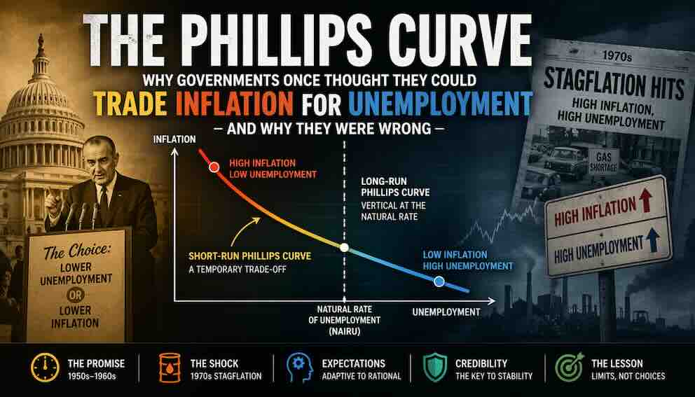
A Conceptual Visual Summary: Imagine two diagrams. In the first diagram, the short-run Phillips Curve is a downward-sloping line. A point on that line shows a combination of inflation and unemployment. If the government uses expansionary policy, the economy moves up and left along that line – lower unemployment, higher inflation. But then expected inflation rises, and the entire short-run curve shifts up. The economy ends up with higher inflation and the same unemployment as before. In the long run, after repeated shifts, the only points that remain are those where unemployment equals the natural rate. Connect those points, and you get a vertical line. That vertical line is the long-run Phillips Curve. In the second diagram, imagine a supply shock – an oil price spike. This adds directly to inflation (the +s term in the equation). The short-run curve shifts up, but the natural rate does not change. The result is higher inflation and, depending on how the central bank responds, potentially higher unemployment as well. That is stagflation.

Key Takeaway – Long-Run Phillips Curve: The LRPC is vertical at the natural rate of unemployment (NAIRU). There is no long-run trade-off. Any attempt to keep unemployment below the natural rate leads only to accelerating inflation, not permanently lower unemployment.

The Breakdown – Stagflation and the Role of Supply Shocks

If the simple Phillips Curve trade-off had continued to work, the 1970s would have looked very different. But the 1970s delivered something that the original Phillips Curve said was impossible: high inflation and high unemployment at the same time. This combination was given a grim name – stagflation, a portmanteau of stagnation (high unemployment, low growth) and inflation. And stagflation broke the simple Phillips Curve.

In 1973, the Yom Kippur War led to an oil embargo by Arab oil-producing countries against nations that supported Israel. The price of oil quadrupled almost overnight. Then, in 1979, the Iranian Revolution caused another oil shock, and oil prices doubled again. These were supply shocks – sudden, sharp increases in the cost of a key input to production. In our expectations-augmented equation, these supply shocks appear as the +s term. A large positive supply shock adds directly to inflation, regardless of what is happening to unemployment. The result is that both inflation and unemployment can rise together – exactly what happened in the 1970s.

The United States experienced this painfully. In 1973, unemployment was about five per cent and inflation was about six per cent. By 1975, after the first oil shock, unemployment had jumped to nine per cent and inflation had soared to twelve per cent. By 1980, after the second oil shock, unemployment was over seven per cent and inflation had hit fourteen per cent. The United Kingdom fared even worse. In 1975, inflation peaked at over twenty-five per cent while unemployment was also rising sharply. The simple trade-off had vanished. But note: the expectations-augmented Phillips Curve with a supply shock term predicts exactly this outcome. The failure was not of the modern model but of the simple, expectations-free version that policymakers had been using.

What went wrong with the original Phillips Curve? The answer is expectations and supply shocks. As inflation rose year after year, workers and businesses revised their expectations upward. They no longer believed that inflation would return to two per cent. They began to expect high inflation as the new normal. This shift in expectations – an increase in π^e – caused the short-run Phillips Curve to shift upward. At every level of unemployment, inflation was higher because people expected higher inflation. Combined with the direct effect of the oil shocks (the +s term), the result was devastating.

Key Takeaway – Stagflation: The 1970s oil shocks caused both inflation and unemployment to rise together. The expectations-augmented Phillips Curve explains this through the supply shock term (+s) and through rising expected inflation (π^e) shifting the curve upward. The simple Phillips Curve failed because it ignored both.

The Role of Expectations – From Adaptive to Rational

The stagflation of the 1970s forced economists to rethink how expectations work. The old view was adaptive expectations: people form their expectations based on past inflation. If inflation was two per cent last year, they expect two per cent this year. If inflation then rises to five per cent, they slowly adjust their expectations over time. This slow adjustment is what creates the short-run trade-off. The government can surprise people with higher inflation, and for a while, unemployment falls because workers have not yet demanded higher wages to compensate.

But the 1970s showed that expectations could adjust much faster than the adaptive expectations model predicted. Workers and businesses did not wait patiently for inflation to prove itself year after year. They saw the oil shocks, they saw the money supply expanding, and they revised their expectations immediately. This led to the development of the rational expectations hypothesis, most closely associated with economist Robert Lucas. Rational expectations means that people use all available information – not just past inflation, but also current policy announcements, oil price movements, and their understanding of how the economy works – to form their expectations. They are not systematically fooled by policymakers.

In the extreme version of rational expectations, even the short-run trade-off disappears. When the government announces an expansionary policy, people immediately anticipate the higher inflation that will result. Workers demand higher wages right away. Businesses raise prices right away. The increase in aggregate demand leads directly to higher inflation, with no temporary reduction in unemployment. The Phillips Curve becomes vertical even in the short run. However, most economists today believe this extreme version is not accurate. Prices and wages are sticky – they do not adjust instantly. Information is imperfect – not everyone knows what the central bank is planning. So most mainstream economists believe that a short-run trade-off still exists, but it is weaker and less exploitable than the original Phillips Curve suggested. The rational expectations critique did not kill the Phillips Curve, but it forced economists to take expectations seriously and to recognise that the trade-off could be much smaller than previously thought.

Key Takeaway – Expectations Matter: Adaptive expectations (based on past inflation) create a short-run trade-off. Rational expectations (using all available information) suggest the trade-off may be very small or zero. Most economists take a middle view: a short-run trade-off exists but is weak, and policy credibility is essential.

Policy Credibility and the Sacrifice Ratio

If expectations matter so much, then the most important thing a central bank can have is credibility. Credibility means that the public believes the central bank will do what it says. If the central bank has a two per cent inflation target and the public believes it will achieve that target, then inflation expectations π^e will anchor at two per cent. Workers will demand wage increases of about two per cent. Businesses will raise prices by about two per cent. Inflation will stay near two per cent, even without constant active intervention. And crucially, when a supply shock hits, anchored expectations mean that the shock does not spiral into persistent high inflation.

Building credibility is hard. It took Paul Volcker, the Chairman of the Federal Reserve from 1979 to 1987, years of painful high interest rates to convince the American public that inflation would be controlled. In 1979, inflation was over thirteen per cent. Volcker raised the federal funds rate – the key interest rate controlled by the Fed – to nearly twenty per cent. This caused a deep recession. Unemployment rose to nearly eleven per cent in 1982. But Volcker did not back down. He kept rates high until inflation fell. By 1983, inflation was under four per cent. And crucially, the public now believed that the Fed would keep it low. That credibility has persisted, with some wobbles, for forty years.

The cost of reducing inflation is measured by the sacrifice ratio. The sacrifice ratio tells us how much output or unemployment must be sacrificed to reduce inflation by one percentage point. In the early 1980s, the sacrifice ratio was high – the Volcker disinflation caused a deep recession that cost many jobs and much lost output. But the alternative – allowing high inflation to continue – would have been even worse in the long run. The sacrifice ratio is not fixed; it depends on how credible the central bank is. A credible central bank can reduce inflation with a much smaller recession because expectations adjust quickly. A central bank with no credibility must cause a deep recession to convince the public that it is serious. This is why building credibility is so valuable. It lowers the sacrifice ratio.

The importance of credibility became clear again after the COVID-19 pandemic. When inflation surged to nine per cent in the United States and eleven per cent in the United Kingdom, central banks had to act. But because they had built credibility over decades, they could raise interest rates gradually and the public believed they would bring inflation back down. Inflation expectations did not become unanchored. People did not start expecting ten per cent inflation year after year. That credibility allowed central banks to fight inflation without causing a complete economic collapse. The sacrifice ratio in the post-COVID disinflation appears to have been much lower than in the 1980s because expectations remained anchored. In contrast, countries without credible central banks – like Argentina or Turkey – saw inflation expectations spiral out of control, making the problem much worse and forcing much higher sacrifice ratios.

Key Takeaway – Policy Credibility and the Sacrifice Ratio: If the public believes the central bank will control inflation, expectations anchor at the target. This makes it easier to keep inflation low without causing recessions. The sacrifice ratio measures the cost of reducing inflation. Credible central banks have lower sacrifice ratios because expectations adjust quickly.

The Modern Phillips Curve – Flat, Nonlinear, and Anchored

Is the Phillips Curve dead? After the 1970s, many economists declared it dead. But then something interesting happened. From the mid-1980s until the COVID-19 pandemic, the Phillips Curve seemed to re-emerge, but in a much flatter form. In the 1990s and 2000s, when unemployment fell in the United States and the United Kingdom, inflation rose only modestly. When unemployment rose during recessions, inflation fell only modestly. The relationship was weaker than Phillips had found in the 1950s, but it was still there.

What explains this flatter relationship? Several factors. First, globalisation has made inflation less sensitive to domestic unemployment. When a country's unemployment rises, it can still import cheap goods from China or Vietnam, so prices do not fall as much. Second, central bank credibility has anchored inflation expectations. When people believe the central bank will keep inflation near two per cent, they do not change their expectations much even when unemployment fluctuates. This anchors the Phillips Curve, making it flatter. Third, the structure of the labour market has changed, with more part-time and gig economy jobs that do not create the same wage pressure as traditional full-time employment.

The COVID-19 pandemic and its aftermath have reminded us that the Phillips Curve is not dead, but it is nonlinear. It is very flat at normal times, meaning that small changes in unemployment produce very small changes in inflation. But when the economy overheats dramatically – when unemployment falls far below the natural rate – the curve can become steep. When unemployment fell to historically low levels in 2022 and 2023 – below four per cent in the United States – inflation surged. The trade-off reasserted itself, but only after a massive, once-in-a-century shock. This nonlinearity is a major insight in current macroeconomics. The Phillips Curve is not a stable line that policymakers can rely on. It is a relationship that changes depending on how far the economy is from the natural rate and how well-anchored expectations are.

Key Takeaway – The Modern Phillips Curve: The modern Phillips Curve is flatter than in the past due to globalisation, anchored expectations, and labour market changes. It is also nonlinear – very flat at normal times but steeper when the economy overheats. The post-COVID inflation surge showed that the trade-off still exists, but only at very low unemployment levels.

Conclusion: The Phillips Curve Teaches Us About Limits

The history of the Phillips Curve is a story of discovery, hubris, failure, learning, and rediscovery. It began as a simple empirical observation – a downward-sloping line on a scatter plot – that seemed to offer governments a menu of choices. For a decade, policymakers believed they could trade higher inflation for lower unemployment, and they acted on that belief. Then the 1970s delivered stagflation, and the simple trade-off shattered. Economists had to go back to first principles. The result was one of the most important advances in macroeconomics: the expectations-augmented Phillips Curve, with its equation π = π^e − β (u − u^*) + s. This equation teaches us that the short-run trade-off depends on expectations being slow to adjust, that the long-run Phillips Curve is vertical at the natural rate, and that supply shocks can break the relationship entirely. It also teaches us the accelerationist insight: to keep unemployment below the natural rate, inflation must keep rising year after year. The Phillips Curve is not a policy menu. It is a constraint. It tells policymakers that they cannot fool all of the people all of the time. They can surprise workers and businesses with unexpected inflation, and for a brief moment, unemployment will fall. But once expectations adjust, the economy returns to the natural rate, now with higher inflation. The only lasting way to reduce unemployment is to improve the real functioning of the labour market – through education, training, and reform. The Phillips Curve does not give governments a free lunch. It gives them a lesson in humility. And that lesson, learned at great cost in the 1970s and reinforced by the post-pandemic inflation surge, remains one of the most important ideas in all of macroeconomics.