Labour Market Dynamics Explained: Job Flows, the Matching Function, and the Beveridge Curve – A Complete Macroeconomics Guide

Why Labour Markets Are Always Moving – Job Flows and the Stock-Flow Distinction

When people think about the labour market, they often imagine a simple picture: some people have jobs, and some people do not. If unemployment is low, the economy is doing well. If unemployment is high, the economy is struggling. While this is not incorrect, it is far too simplistic to capture what is actually happening beneath the surface. Even in a healthy and stable economy where unemployment appears low and steady, there is a constant process of jobs being created and jobs being destroyed. Firms expand and hire new workers, while others downsize or shut down. Workers leave jobs voluntarily, are laid off, or move to better opportunities. This continuous movement is what economists refer to as labour market dynamics.

To understand this properly, we need to distinguish between stocks and flows – a distinction that is fundamental to all of macroeconomics. The unemployment rate is a stock: it measures how many people are unemployed at a particular point in time, like a photograph of the labour market on a specific day. However, this stock is constantly changing because of flows – movements of people between employment, unemployment, and being outside the labour force. Workers flow into unemployment when they lose jobs (a flow called job destruction). Workers flow out of unemployment when they find new jobs (a flow called job creation). The unemployment rate at any moment is therefore determined not just by how many jobs exist, but by how quickly workers are losing jobs and how quickly unemployed workers are finding new ones. A stable unemployment rate does not mean nothing is changing. It means that the flow into unemployment and the flow out of unemployment are balanced.

Job creation refers to the process by which firms generate new employment opportunities. A company may expand production because demand for its products has increased. A new firm may enter the market and begin hiring workers. Technological innovation can also create entirely new industries. For example, consider the rise of the renewable energy sector over the past two decades. As governments and consumers have shifted toward cleaner energy sources, companies involved in solar and wind energy have expanded rapidly, creating new jobs for engineers, technicians, and construction workers – jobs that did not exist in significant numbers thirty years ago. Job destruction is the opposite process. A clear example can be seen in the decline of traditional retail jobs due to the growth of online shopping. As consumers increasingly purchase goods through digital platforms like Amazon, many physical retail stores have closed, leading to job losses for cashiers, shelf-stackers, and store managers. Between 2010 and 2020, the United States lost over 60,000 retail jobs despite a growing economy, while e-commerce jobs grew by more than 200,000.

One of the most important insights in modern macroeconomics is that job creation and job destruction are happening all the time, even when the economy appears stable. In a typical month in a developed economy, millions of jobs may be created while millions of others are destroyed. Imagine an economy where 1 million jobs are created in a month and 1 million jobs are destroyed. The net change in employment is zero, so the unemployment rate remains unchanged. However, beneath this stable surface, there is significant movement as workers transition between jobs or between employment and unemployment. Job flows are crucial because they reveal the underlying health and flexibility of the labour market. A dynamic labour market with high job creation and destruction can indicate that resources are being reallocated efficiently. Workers move from less productive jobs to more productive ones, and firms adapt to changing economic conditions. If job destruction consistently exceeds job creation, unemployment will rise. If job creation outpaces job destruction, employment will grow.

But job creation and destruction alone do not determine employment outcomes. What matters equally is how efficiently workers and firms can find each other. This brings us to the matching function.

Key Takeaway – Stocks and Flows: Unemployment is a stock (a point-in-time measure). Job creation and destruction are flows that change that stock. A stable unemployment rate hides constant movement. The separation rate (workers losing jobs) and the job-finding rate (workers finding jobs) together determine unemployment dynamics.

The Matching Function – How Workers and Firms Find Each Other Despite Search Frictions

Once jobs are created and workers become unemployed, the next crucial question is: how do workers and firms find each other? This process is not automatic or instantaneous. It involves searching, interviewing, evaluating, and negotiating. In the real world, information is imperfect, workers do not know about every vacancy, and firms do not know about every job seeker. These obstacles are called search frictions (or matching frictions), and they are the reason why unemployment and vacancies can coexist. Economists model this process using the matching function.

The matching function is usually written as M = f(U, V), where M is the number of successful matches (workers who find jobs and firms who fill vacancies), U is the number of unemployed workers actively seeking jobs, and V is the number of job vacancies (open positions that firms are trying to fill). The function tells us that the number of matches depends on both the number of unemployed workers and the number of vacancies. The more vacancies there are, the easier it is for workers to find jobs. The more unemployed workers there are, the easier it is for firms to find suitable candidates. However, the relationship is not one-to-one. Doubling U and V does not necessarily double M, because search frictions remain. There can be mismatches in skills, location, or information.

From the matching function, we can derive two crucial rates. The job-finding rate (f) is the probability that an unemployed worker finds a job in a given period. It is calculated as f = M/U. The separation rate (s) is the probability that an employed worker loses their job in a given period. The unemployment rate in the long run tends toward the steady-state level given by u = s / (s + f). This simple equation is one of the most powerful in labour economics. It tells us that unemployment is high when the separation rate is high (workers lose jobs quickly) or when the job-finding rate is low (unemployed workers struggle to find new jobs). Even if job destruction is high, unemployment may remain low if workers quickly find new jobs – that is, if the job-finding rate is also high.

From the matching function, economists also derive a concept called labour market tightness, denoted by the Greek letter theta (θ). Labour market tightness is the ratio of vacancies to unemployment: θ = V/U. When V is high relative to U, the labour market is tight. There are many jobs chasing few workers. In this situation, workers have bargaining power – they can demand higher wages, better conditions, and they can switch jobs easily. When U is high relative to V, the labour market is slack. There are many workers chasing few jobs. Employers have bargaining power – they can offer lower wages and workers have few alternatives.

Crucially, labour market tightness directly affects wages. When the labour market is tight (high θ), firms compete for scarce workers by offering higher wages. This puts upward pressure on wage growth, which in turn can feed into inflation. When the labour market is slack (low θ), workers compete for scarce jobs, which puts downward pressure on wages. This is why central banks monitor labour market tightness so closely – it is a key indicator of future wage inflation and, ultimately, price inflation. The post-COVID recovery saw record tightness in many economies, with vacancies exceeding unemployment for the first time in decades, contributing to the inflation surge of 2021-2023.

Key Takeaway – Matching Function and Key Rates: The matching function M = f(U, V) describes how matches occur despite search frictions. The job-finding rate (f = M/U) and separation rate (s) determine the steady-state unemployment rate: u = s/(s+f). Labour market tightness θ = V/U determines worker bargaining power and wage pressures.

The Beveridge Curve – Linking Vacancies and Unemployment

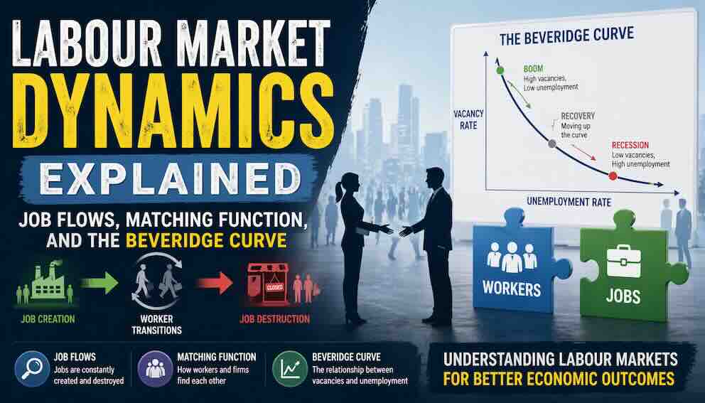
The Beveridge Curve, named after the British economist William Beveridge, is one of the most important tools in labour economics. It shows the empirical relationship between job vacancies and unemployment. Imagine a graph where the horizontal axis represents the unemployment rate and the vertical axis represents the vacancy rate (the number of vacancies as a share of the labour force). The curve slopes downward from the top left to the bottom right. Each point on the curve represents a particular state of the labour market at a point in time.

The Beveridge Curve is downward sloping for a clear reason. When unemployment is high, vacancies tend to be low. In a recession, firms reduce production and cut back on hiring. Many workers lose their jobs, leading to high unemployment. At the same time, firms post fewer job vacancies because they are uncertain about the future. This results in a point on the Beveridge Curve with high unemployment and low vacancies – the bottom right of the curve. When the economy booms, the situation is reversed. Firms expand production and actively seek workers, leading to a high number of vacancies. At the same time, more workers find jobs, so unemployment falls. This results in a point on the Beveridge Curve with low unemployment and high vacancies – the top left of the curve.

A concrete example from history helps make this concrete. After the global financial crisis of 2008, many economies experienced a sharp increase in unemployment along with a decline in job vacancies. In the United States, the unemployment rate rose from 4.4 per cent in early 2007 to 10 per cent in late 2009, while the vacancy rate fell sharply. This placed the US economy at a point on the Beveridge Curve characterised by high unemployment and low vacancies. During the recovery phase from 2010 to 2019, job vacancies increased while unemployment gradually declined, moving the economy along the curve in the opposite direction – up and to the left, towards low unemployment and high vacancies.

Key Takeaway – Beveridge Curve (Movements): The Beveridge Curve slopes downward from top left (low unemployment, high vacancies) to bottom right (high unemployment, low vacancies). Movements along the curve reflect the business cycle: recessions move to the bottom right; booms move to the top left.

The Microfoundation – How the Beveridge Curve Emerges from the Matching Function

The Beveridge Curve is not just an empirical observation. It can be derived directly from the matching function, which gives it a solid theoretical foundation. Understanding this derivation is important because it shows why the curve is stable in normal times and why it shifts when matching efficiency changes.

Recall the matching function M = f(U, V). The job-finding rate is f = M/U. In steady state, the unemployment rate is determined by u = s/(s+f). For a given level of vacancies V, a better matching function (higher M for the same U and V) means a higher job-finding rate f, which means lower unemployment u. Conversely, if matching efficiency deteriorates, f falls and u rises for the same V. Now, plot different combinations of u and V that satisfy the steady-state condition for a given matching efficiency. As V increases, f increases, and u decreases. This generates a downward-sloping curve in (u, V) space. That curve is the Beveridge Curve. The exact position of the curve depends on the efficiency of the matching function. A more efficient matching function (one that produces more matches from the same U and V) shifts the Beveridge Curve inward (toward the origin). A less efficient matching function shifts it outward.

This microfoundation is not just academic. It tells us that the Beveridge Curve is not a fixed law of nature. It shifts when matching efficiency changes – when search frictions become more or less severe. This is why we need to distinguish between movements along the curve (which reflect changes in V driven by the business cycle) and shifts of the curve (which reflect changes in matching efficiency).

Key Takeaway – Microfoundation: The Beveridge Curve is derived from the matching function and the steady-state unemployment condition. A more efficient matching function shifts the curve inward (lower unemployment for given vacancies). A less efficient matching function shifts it outward.

Shifts in the Beveridge Curve – What They Reveal About Structural Unemployment

The most important insight from the Beveridge Curve comes not from movements along the curve but from shifts of the curve itself. A shift of the curve indicates that the relationship between vacancies and unemployment has changed. For the same level of vacancies, unemployment is higher or lower than before. This tells us something profound about the underlying efficiency of the labour market – specifically, about the severity of search frictions.

An outward shift of the Beveridge Curve means that for any given level of vacancies, unemployment is higher than before. The curve has moved away from the origin. This suggests that the labour market has become less efficient at matching workers with jobs. Search frictions have increased. Why might this happen? The most common causes are skills mismatch (workers do not have the skills required for the available jobs), geographic mismatch (jobs are located in different regions than where unemployed workers live), and long-term unemployment (workers who have been unemployed for a long time lose skills or become less attractive to employers, making them harder to place). An outward shift is bad news. It means that even when the economy recovers and vacancies return to normal levels, unemployment will remain higher than before because the matching process is broken.

An inward shift of the Beveridge Curve means that for any given level of vacancies, unemployment is lower than before. The curve has moved toward the origin. This suggests that the labour market has become more efficient. Search frictions have decreased. Factors that can improve matching efficiency include better education and training systems (workers have the skills employers need), improved job search technologies (online platforms like LinkedIn and Indeed that connect workers and firms quickly), greater mobility of workers (people are willing and able to move to where jobs are), and effective labour market policies (like retraining programmes for displaced workers). An inward shift is good news. It means that the economy can achieve lower unemployment without needing as many vacancies.

The best real-world example of an outward shift occurred in Spain after the 2008 financial crisis. Before the crisis, Spain's Beveridge Curve was relatively close to the origin. But after the crisis, the curve shifted outward dramatically. Even as vacancies began to recover, unemployment remained stubbornly high – above 20 per cent for years. Why? Because Spain had a severe skills mismatch. The jobs that were being created were in technology and services, but the workers who had lost jobs were in construction. Those construction workers did not have the skills for the new jobs, and Spain's training system was slow to adapt. Search frictions increased dramatically. This outward shift reflected a deep structural problem that could not be solved simply by stimulating demand. In contrast, the United States experienced a smaller outward shift, and its Beveridge Curve returned closer to its original position as the recovery progressed, reflecting a more flexible labour market with lower search frictions.

More recently, during the COVID-19 pandemic, many countries experienced temporary outward shifts as lockdowns disrupted matching. But as economies reopened and online job matching improved, some countries saw partial inward shifts. The United Kingdom, for example, saw vacancies surge to record levels in 2022, with more vacancies than unemployed workers for the first time on record – an extremely tight labour market that moved the economy to the top left of the curve.

Key Takeaway – Beveridge Curve Shifts: An outward shift (worse matching, higher search frictions) means higher unemployment for any given level of vacancies – caused by skills mismatch, geographic mismatch, or long-term unemployment. An inward shift (better matching, lower search frictions) means lower unemployment. Shifts reveal structural problems that demand-side policies cannot fix.

Bringing It All Together – A Complete Picture of Labour Market Dynamics

We can now see how all the pieces fit together. Labour markets are constantly in motion, with jobs being created and destroyed every month. This churn is not a sign of instability; it is a sign of a dynamic economy where resources are reallocated from declining sectors to growing ones. The unemployment rate is a stock, but it is changed by flows – the separation rate (workers losing jobs) and the job-finding rate (workers finding jobs). The matching function M = f(U, V) describes how unemployed workers and job vacancies find each other despite search frictions. Labour market tightness θ = V/U determines who has bargaining power and, through that, wage growth and inflation pressures. The Beveridge Curve plots the empirical relationship between unemployment and vacancies, showing a downward slope that reflects the business cycle. Movements along the curve tell us about booms and recessions. But shifts of the curve tell us something deeper: whether search frictions have increased or decreased – that is, whether the labour market has become more or less efficient at matching workers to jobs. An outward shift – like the one Spain experienced after 2008 – indicates structural problems like skills mismatches that require training and reform, not just stimulus. An inward shift – driven by better job matching technology like online platforms – indicates improved efficiency.

For students and policymakers alike, the key insight is this: not all unemployment is the same. Some unemployment is cyclical – it rises in recessions and falls in booms, and it can be addressed by increasing aggregate demand. But some unemployment is structural – it persists even when vacancies are available because workers and jobs do not match, because search frictions are severe. The Beveridge Curve, by distinguishing movements from shifts, gives us a powerful tool to tell these two types apart. When unemployment rises but the economy stays on the curve, the problem is cyclical. When the curve shifts outward, the problem is structural. And the solution must match the diagnosis: demand stimulus for cyclical problems, but training, mobility, and matching improvements for structural problems.

Conclusion: Seeing the Labour Market as a Dynamic System with Frictions

Labour markets are not static systems where jobs simply exist and workers fill them instantly. Instead, they are constantly evolving environments characterised by continuous job creation and destruction, ongoing search and matching processes despite unavoidable frictions, and complex relationships between vacancies and unemployment that change over time. By understanding job flows, we gain insight into the underlying movements that shape employment levels. Through the matching function, we see how the interaction between workers and firms determines the job-finding rate and, together with the separation rate, the steady-state unemployment rate. The Beveridge Curve then provides a visual framework to interpret these dynamics, while shifts in the curve reveal deeper structural changes in the economy – changes that demand structural solutions rather than simple demand stimulus. When all these elements are considered together, it becomes clear that unemployment is not just a simple number but the result of multiple interacting forces: the rate at which jobs are destroyed, the rate at which workers find new jobs, the tightness of the labour market, and the efficiency of the matching process. A deeper understanding of these forces allows economists and policymakers to design better strategies: training programmes for workers whose skills no longer match available jobs, relocation assistance for workers stuck in regions without employment, and better matching technology to speed up the search process. The goal is not to eliminate job flows – that would be impossible and undesirable – but to reduce search frictions so that the matching process works efficiently. When matching works well, unemployment is as low as possible, as brief as possible, and as fair as possible. That is the promise of labour market dynamics, and the Beveridge Curve is the compass that helps us navigate the journey.