Keynesian Consumption Function Explained: Formula, MPC, Examples, and Real-World Economic Behavior

Introduction: The Quiet Decisions We Make Every Day

Every month, households across the country face the same quiet question. The paycheck arrives. The bills are due. How much to spend? How much to set aside?

These decisions seem personal. They feel like matters of habit and discipline. But when millions of households make these choices at the same time, they shape the entire economy. Spending drives production. Production drives employment. Employment drives income. And income, in turn, drives more spending.

Understanding this relationship helps explain why governments intervene during recessions and how economic shocks spread through the economy.

In the 1930s, the economist John Maynard Keynes offered a simple but powerful way to understand this cycle. He argued that the most important factor determining how much people spend is how much money they have right now. Not what they hope to earn next year. Not what they saved ten years ago. Their current income.

This idea became known as the Keynesian Consumption Function. It is not a complete theory of household behavior. But it is a foundation. And understanding it is the first step toward understanding how economies grow, why recessions happen, and how governments try to help.

When This Model Works Best: The Short Run

The Keynesian Consumption Function is designed for the short run. This matters because it tells us when the model is most useful.

In the short run, people cannot easily adjust their long-term plans. They cannot immediately move to a cheaper city when income falls. They cannot instantly retrain for a better job. They respond to changes in income with the tools they have: spending a bit more, saving a bit less, or borrowing.

This makes the Keynesian model particularly relevant during recessions or periods of sudden income change. When a factory closes and workers lose their jobs, they do not stop spending entirely. They cut back where they can, but they still pay rent and buy food. When a household receives an unexpected bonus, they do not save every pound. They treat themselves to something.

Governments use this model for short-term policy design. When designing a stimulus package, they want to know how much of each pound given to households will be spent. The answer depends on the marginal propensity to consume, which tends to be higher for lower-income households.

Later in this tutorial, we will discuss why the model works less well for long-term planning. But for understanding how households react to immediate changes in income, the Keynesian framework remains essential.

The Core Idea: People Spend What They Have

Keynes started with an observation that seems almost too obvious. People spend money when they have money. When income rises, spending rises. When income falls, spending falls.

But he noticed something more subtle. Spending does not rise or fall by the same amount as income. When a household receives a raise, it does not spend every extra pound. It saves some. When a household takes a pay cut, it does not reduce spending by the full amount. It dips into savings or borrows.

This simple observation became the heart of the Keynesian Consumption Function. Current income drives spending. But the relationship is not one-to-one.

To understand why, consider a factory worker named Carol. She works at an automobile plant in the English Midlands. Her take-home pay is £2,200 per month after taxes. She spends most of it on rent, groceries, utilities, and transportation. She saves a small amount each month, perhaps £150, for emergencies or future plans.

Now imagine Carol receives a promotion. Her monthly pay rises to £2,500, an increase of £300. What does she do with the extra money? She might spend some of it. Perhaps she upgrades her mobile phone or eats out more often. But she will almost certainly save some of it as well.

If Carol spends £200 of the £300 raise and saves £100, her marginal propensity to consume is 0.67. For every additional pound of income, she spends about 67 pence and saves 33 pence.

This is not a theory about Carol's personal habits. It is a pattern that holds across millions of households. People with higher incomes spend more, but they also save more. And as incomes rise, the share of income that is saved tends to increase.

The Equation: A Simple Mathematical Home

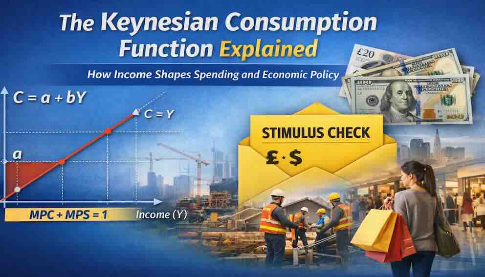
The Keynesian Consumption Function can be written as a simple equation:

C = a + bYd

This looks abstract, but each piece stands for something real.

C stands for total consumption. That is everything households spend on goods and services: rent, groceries, petrol, dinners out, streaming subscriptions, school fees.

Yd stands for disposable income. That is income after taxes. It is the money households actually have available to spend or save.

a stands for autonomous consumption. This is the spending that happens independently of income. It has two important sources. First, even when income is zero, people still need to consume. They use savings, borrow, or receive help from family or government. A student living on loans, a retired person drawing down savings, a family receiving unemployment benefits—all are consuming without current earned income.

Second, some spending is not optional. Rent obligations, basic food consumption, and contractual payments must be made regardless of income level. Autonomous consumption captures this reality. It is the baseline spending that does not disappear even when times are hard.

b stands for the marginal propensity to consume, often shortened to MPC. This is the fraction of each additional pound of income that goes to consumption. If the MPC is 0.75, then for every extra £1 of income, consumption rises by 75 pence. The remaining 25 pence is saved.

The MPC is always between 0 and 1. It cannot be negative because people do not reduce consumption when income rises. It cannot exceed 1 because people do not spend more than the extra income they receive.

Understanding MPC and the Other Half: Saving

The marginal propensity to consume becomes clearer when connected to everyday decisions. Suppose a person receives a £100 bonus at work. Instead of spending the entire amount, they might spend £70 and save £30. In this case, the MPC is 0.7, because 70 percent of the additional income is used for consumption.

The portion of income that is not consumed is saved. This leads to the marginal propensity to save, or MPS. In the same example, the MPS would be 0.3, because £30 out of £100 is saved.

The two always add up to one:

MPC + MPS = 1

This is not a theory. It is an accounting identity. Every pound of income has only two places to go. It is either spent or saved. There is no third option.

This simple relationship has powerful implications. If economists can measure how much people spend when income rises, they automatically know how much people save. And if they know the MPC, they can predict how a tax cut or a government stimulus will affect the economy.

A higher MPC means that extra income flows quickly into spending, which boosts production and employment. A lower MPC means that extra income leaks into savings, dampening the impact on the wider economy.

Average Propensity to Consume: A Related Concept

The marginal propensity to consume tells us what happens at the edge. It answers the question: when income changes by one pound, how much does consumption change?

But there is another useful measure. The average propensity to consume, or APC, tells us what share of total income is spent on consumption. The formula is simple:

APC = C / Yd

If a household earns £2,000 per month and spends £1,800, the APC is 0.9. The household spends 90 percent of its income and saves 10 percent.

The APC tends to fall as income rises. Lower-income households spend most of what they earn because they have little room to save. Higher-income households save a larger share. This pattern is exactly what Keynes observed, and it is why the consumption function is flatter than the 45-degree line.

The distinction between marginal and average propensity matters for policy. A household with a high MPC will respond strongly to a temporary tax cut. But its APC might still be high because most of its income goes to necessities. The two measures tell different but related stories.

Visualizing the Relationship: The 45-Degree Line

Imagine a simple graph. On the bottom line, from left to right, we measure disposable income. On the vertical line, going up, we measure consumption.

Now imagine a straight line running from the bottom left to the top right at a 45-degree angle. Every point on this line represents a situation where consumption equals income. If a household is on this line, it is spending every pound it earns and saving nothing.

The consumption function is also a straight line rising from left to right. But it is flatter than the 45-degree line. It does not start at zero. It starts at the level of autonomous consumption, the spending that happens even with no income.

The gap between the 45-degree line and the consumption function represents saving. When the consumption line is below the 45-degree line, households are saving. When the consumption line is above it, which can happen at very low income levels, households are dissaving, meaning they are spending more than they earn by drawing down savings or borrowing.

As income grows, the gap between the two lines widens. This reflects the fact that people with higher incomes save a larger share. The slope of the consumption function is the MPC. A steeper slope means a higher MPC. A flatter slope means a lower MPC.

A Real-World Anchor: The Early 1990s Recession

To see the Keynesian Consumption Function in action, consider the recession of the early 1990s in the United Kingdom. The economy contracted sharply. Unemployment rose. Many households saw their incomes fall.

What happened to spending? It fell. But it did not fall as much as income. Households tried to protect their living standards. They reduced their savings. They borrowed more. They cut back on luxuries but kept paying for essentials.

This behavior matches the Keynesian model perfectly. When income falls, consumption falls too, but not by the same amount. The MPC during a downturn is still positive, but the relationship works in both directions.

Now consider the recovery that followed. As incomes slowly rose again, households did not spend all of their new income. They used some of it to rebuild savings that had been depleted during the recession. The MPC during the recovery was less than one, just as Keynes predicted.

The pattern holds across decades. Income goes up. Spending goes up, but less than income. Income goes down. Spending goes down, but less than income. The relationship is stable enough to be useful, even if it is not perfectly precise.

Why Governments Care About the MPC

The marginal propensity to consume is not just an abstract concept. It directly shapes how governments design economic policy.

When a government wants to stimulate a struggling economy, it can put money into the hands of households through tax cuts or direct payments. But not every household will spend that money. Some will save it. The effectiveness of the stimulus depends on the MPC.

Households with lower incomes tend to have higher MPCs. They have less room to save because most of their income already goes to necessities. A £100 payment to a low-income household is likely to be spent quickly on rent, food, or repairs. A £100 payment to a high-income household might simply be added to savings.

This is why many stimulus programs target lower-income households. Policymakers understand that the same amount of money generates more spending when it goes to those who are most likely to spend it. The Keynesian Consumption Function provides the theoretical foundation for this intuition.

The same logic applies to tax cuts. A tax cut that benefits lower-income households will generate more immediate spending than a tax cut that benefits higher-income households. The MPC tells policymakers where their money will have the greatest impact.

Where the Model Falls Short

The Keynesian Consumption Function is a powerful starting point. But it is not the final word.

One limitation is that it focuses only on current income. In reality, people look ahead. A young doctor with low current income but high future earnings might spend more than her income suggests. A factory worker expecting a layoff might save more. Expectations about the future matter.

Another limitation is that it does not explain why consumption is so stable over time. In real economic data, consumption rises and falls much less than income. People smooth their spending. They save in good times and borrow in bad times to keep their consumption relatively steady. Keynes acknowledged this but did not fully incorporate it into his model.

This is where later economists built on Keynes's foundation. Franco Modigliani developed the life-cycle hypothesis, which argues that people plan their consumption over their entire lifetime, saving during their working years and spending during retirement. Milton Friedman developed the permanent income hypothesis, which distinguishes between temporary changes in income and permanent changes. A temporary bonus might be mostly saved, while a permanent raise might lead to a lasting increase in consumption.

These later theories do not reject Keynes. They extend him. Keynes explains immediate behavior. Modigliani and Friedman explain planning over time. Together, they provide a fuller picture of how households make decisions.

Yet the Keynesian framework remains essential. It is the first lesson in how households respond to changes in income. And for understanding recessions, stimulus, and the business cycle, it is still remarkably useful.

Conclusion: A Foundation, Not a Final Answer

The Keynesian Consumption Function teaches a simple but powerful lesson. People spend based on what they have right now. When income rises, spending rises, but not by the full amount. When income falls, spending falls, but not by the full amount. The difference is saving.

This relationship, captured in the equation C = a + bYd, gives economists a way to predict how households will respond to tax changes, government spending, and economic booms or busts. The marginal propensity to consume is the key that unlocks these predictions.

The average propensity to consume adds another layer, showing that higher-income households save a larger share of their income. The 45-degree line helps visualize the gap between income and spending.

But the model is not perfect. It works best in the short run, when households cannot easily adjust their long-term plans. It overlooks expectations, wealth, and the human tendency to smooth consumption over time. Later theories filled in these gaps. Yet none of them would exist without Keynes's original insight.

Understanding the consumption function means understanding that economics is not about perfect predictions. It is about useful approximations. Households do not follow formulas. But they do follow patterns. And the pattern Keynes identified—spending follows income, but not pound for pound—is one of the most durable patterns in all of economics.